Electricity-related emissions accounting is defined under the Greenhouse Gas Protocol (GHG Protocol), the internationally recognized framework for reporting indirect emissions from purchased electricity.
Today, Scope 2 emissions are typically calculated using annual electricity consumption and annual emission factors. As electricity systems evolve and carbon intensity becomes more variable over time, attention is shifting toward whether annual averaging adequately reflects system conditions.
Hourly Scope 2 does not redefine electricity consumption or alter grid operations. What changes is the temporal attribution of emissions. When carbon intensity becomes time-dependent, reported emissions depend not only on how much electricity is consumed, but also on when it is consumed.
Understanding this shift requires revisiting how conventional Scope 2 accounting is structured.
Under the GHG Protocol’s Scope 2 Guidance, organizations calculate emissions by multiplying total electricity consumption over a reporting period by an emission factor associated with the electricity supply:
Annual Scope 2 emissions = Total annual electricity consumption × Annual emission factor
Two approaches are defined:
In both cases, emissions are aggregated over the reporting year. Electricity consumed at different hours is treated equivalently within that annual boundary.
This structure provides comparability and consistency. It also implies temporal aggregation: intraday and seasonal fluctuations in carbon intensity are averaged into a single annual value. Emissions are attributed at the scale of the reporting year, not at the scale at which carbon intensity varies.
Time-dependent Scope 2 accounting applies the same principle but modifies the temporal resolution of the calculation.
Instead of a single annual emission factor, emissions are calculated using carbon intensity values that vary across defined time intervals:
Emissions(t) = Electricity consumption(t) × Carbon intensity(t)
Where:
Total emissions are obtained by summing across all intervals:
Total emissions = Σ Emissions(t)
The reporting boundary remains annual, but attribution becomes time-resolved.
Hourly matching refers to aligning electricity consumption in a given hour with electricity produced in the same region during that hour.
Electricity is treated as time- and region-specific: consuming 1 kWh at 02:00 is not assumed equivalent to consuming 1 kWh at 14:00, and consumption in one region is not assumed equivalent to consumption in another.
In location-based terms, hourly matching asks how consumption relates to regional production conditions at each hour. Where carbon intensity varies significantly, the timing of consumption directly affects attributed emissions.
The key parameter in time-dependent accounting is temporal granularity — the length of the interval used to match consumption and carbon intensity.
As intervals become shorter:
Total electricity use does not change. What changes is how emissions are distributed across time, making results dependent on the organization’s load profile.
Moving from annual averaging to hourly attribution does not change the definition of Scope 2. Electricity remains an indirect emission source.
What changes is the structure of attribution: emissions depend on the interaction between the organization’s load profile and the grid’s carbon intensity at each hour.
Under annual accounting, two organizations with identical annual consumption in the same grid report the same location-based emissions.
Under hourly accounting, this equivalence no longer holds.
Because emissions are calculated as:
Emissions(t) = Consumption(t) × Carbon Intensity(t)
timing becomes decisive. Two entities consuming the same annual kWh may report different emissions if their demand is distributed differently across high- and low-intensity hours.
Total energy remains constant. The load profile becomes an accounting variable.
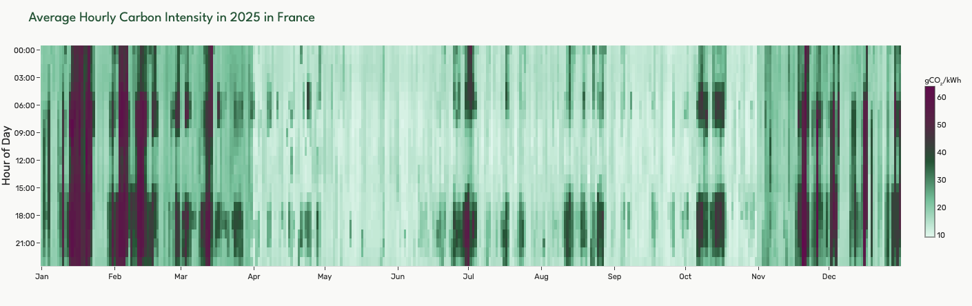
Electricity systems exhibit intraday and seasonal variability in carbon intensity due to changes in generation mix and demand.
Annual averaging smooths this variability. Hourly accounting does not.
Periods of higher carbon intensity contribute proportionally more to reported emissions; lower-intensity periods contribute less. Physical system emissions remain unchanged, but their attribution across time differs.
Interest in hourly Scope 2 reflects structural changes in electricity systems affecting both supply and demand.
Wind and solar generation introduce significant intraday and seasonal variability. Solar peaks during daylight hours; wind fluctuates with weather conditions. As renewable penetration increases, carbon intensity can change markedly within a single day.
In high-renewable systems, midday periods may exhibit lower carbon intensity, while evening peaks require dispatchable fossil generation. The dispersion of hourly values reduces the representativeness of annual averages.
As carbon intensity becomes structurally time-dependent, annual smoothing captures less of operational reality.

High renewable penetration also increases curtailment.
Curtailment occurs when renewable generation cannot be fully utilized because demand is insufficient or network constraints limit transport. This is increasingly observed where significant capacity is connected at the distribution level.
When local production exceeds demand and cannot be exported, renewable output may be reduced despite low-carbon availability. Periods of surplus low-carbon generation can therefore coexist with periods requiring higher-emission dispatch.
Accounting approaches with hourly resolution align more closely with these system dynamics.
Electricity demand is expanding into industry, digital infrastructure, transport, and heating. As electricity becomes a larger share of organizational emissions, the timing of consumption gains importance.
Where carbon intensity fluctuates significantly over the day, the temporal distribution of demand can materially influence reported emissions under time-resolved accounting.
Greater supply variability combined with growing electricity demand makes temporal granularity increasingly relevant in carbon accounting discussions.
Hourly Scope 2 accounting attributes electricity-related emissions based on the carbon intensity of the regional grid at the specific hours when electricity is consumed, making reported emissions dependent on demand timing rather than on annual averages alone.